Last week the LinearModel gained five new methods: feval, coefCI, coefTest, dwtest, and addTerms. This week I went back and fixed a few things that had been sitting quietly wrong, finished the removeTerms companion to addTerms, added support for passing a bare categorical vector directly to fitlm, and then built three plotting methods that let users visually explore what their fitted model is doing.

Project Status

Week 1 was project planning and setup.

Week 2 was the class shell: properties, access rules, the display method, and the subsref gatekeeper.

Week 3 was the constructor and fitlm: the math solver, all the diagnostics, the full 26-property object, and the front-end parser.

Week 4 was applying mentor feedback, refactoring the constructor, and adding predict and random.

Week 5 was a couple of bug fixes and five new public methods: feval, coefCI, coefTest, dwtest, and addTerms.

This week was bug fixes, removeTerms, a new fitlm input form, and three plotting methods.

Bug Fixes

p-value underflow for large t-statistics

The t-test p-values for each coefficient were computed like this:

pval_full(active) = 2 * (1 - tcdf (abs (tstat_full(active)), DFE));

When a predictor fits the data very tightly, the t-statistic becomes a very large number like -43. The old formula asked tcdf for a value very close to 1, then subtracted it from 1. The problem is the computer cannot store enough decimal places to represent that difference, so it rounds to 1 - 1 = 0 and you get a p-value of exactly zero, which is wrong.

pval_full(active) = 2 * tcdf (-abs (tstat_full(active)), DFE);

The fix asks tcdf for the small number directly instead of computing it through subtraction. Same math, but the computer never has to subtract two nearly identical numbers, so the tiny result like 1.2e-28 comes out correctly.

Dfbetas and HatMatrix shape mismatches

The Diagnostics table stores two matrix-valued columns: Dfbetas and HatMatrix.

Dfbetas is an n by p matrix where n is the total number of rows including excluded ones, and p is the number of estimated coefficients. In the previous code, the placeholder was allocated as:

Dfb_full = zeros (n_total, p);   ## was zeros with non-subset rows left as zero

But for non-subset rows, the right value is NaN (not zero), because those rows were never used in the fit so there is nothing meaningful to put there. The fix changes the allocation to NaN and writes the computed values only for the subset rows.

HatMatrix had a different shape problem. The HatMatrix is only computed over the n_obs rows that were actually in the fit, so D.HatMatrix is n_obs by n_obs. The placeholder for the full n_total by n_total padded version was being filled in with the wrong index:

## old - only pads rows, not columns
HatMat_pad(subset_mask, :) = D.HatMatrix;   ## wrong shape

## new - pads both rows and columns correctly
HatMat_pad(subset_mask, subset_mask) = D.HatMatrix;

Power terms in predict

The lm_predict private function handles re-encoding predictor data when you call predict with new inputs. It correctly handled categorical dummy expansion, but for keyword-path models with polynomial terms like 'purequadratic' or 'quadratic', it was only producing the linear column for each predictor and missing the squared columns. Calling predict on a 'purequadratic' model with new data would silently give wrong predictions.

The fix checks the stored EncPredictorNames list for power columns like x1^2, x1^3, and so on, and appends them when they are needed:

function X_enc = lm_predict (X_raw, pred_names, cat_info, enc_names)

The function now accepts the encoded predictor name list as a fourth argument and uses it to detect and generate any power columns during prediction.

Support for bare categorical vectors in fitlm

Previously, if you had a single categorical vector (an Octave categorical array, not a table) and tried to pass it directly to fitlm, you would get an error. The only way to fit a categorical predictor was to put it in a table or pass the numeric codes manually with CategoricalVars.

This week fitlm gained a new entry path at the top that handles this case:

octave:10> Xc = categorical ({'A';'A';'B';'B';'C';'C'});
octave:11> y  = [1.2; 0.9; 2.8; 3.1; 5.0; 4.7];
octave:12> mdl = fitlm (Xc, y)

mdl =

  Linear regression model:
      y ~ 1 + x1

  Coefficients:

  3x4 table

                   Estimate       SE        tStat       pValue       
                   ________    ________    _______    ___________    

    (Intercept)        1.05        0.15          7     0.00598626    
    x1_B                1.9    0.212132    8.95669      0.0029368    
    x1_C                3.8    0.212132    17.9134    0.000379392    


Number of observations: 6, Error degrees of freedom: 3
Root Mean Squared Error: 0.212132
R-squared: 0.990738,  Adjusted R-Squared: 0.984563
F-statistic vs. constant model: 160.444, p-value = 0.000891431

The function converts the categorical vector into a two-column table and then routes it through the existing table path. You can also pass VarNames to control the column names:

mdl = fitlm (Xc, y, 'VarNames', {'group', 'response'})

removeTerms

removeTerms is the mirror of addTerms. You give it the terms you want to remove and it returns a new fitted model with those terms dropped. The original model is never modified.

## remove the interaction term
NewMdl = removeTerms (mdl, 'x1:x2')

## remove a polynomial term
NewMdl = removeTerms (mdl, 'x2^2')

## remove the intercept
NewMdl = removeTerms (mdl, '1')

## remove two terms at once
NewMdl = removeTerms (mdl, 'x1 + x1:x2')

## star operator - removes x1, x2, and their interaction together
NewMdl = removeTerms (mdl, 'x1*x2')

## numeric matrix - each row is a term, columns are predictor exponents
NewMdl = removeTerms (mdl, [1, 1, 0])   ## removes the x1:x2 interaction

Terms you ask to remove that are not in the model are silently skipped. If none of the terms you specified exist in the model, a warning is issued and the original model is returned.

The implementation internally translates the string or matrix you pass into rows of the stored TermsMatrix, removes the matching rows, and calls lm_refit with the result. All the original fit settings - weights, excluded rows, categorical flags - carry over automatically.

## Start from a quadratic model and remove terms one by one
mq  = fitlm (X, y, 'quadratic');
m1  = removeTerms (mq, 'x1:x2');   ## drop interaction
m2  = removeTerms (m1, 'x1^2');    ## drop x1 squared

plotResiduals

plotResiduals visualises the residuals from a fitted model. Residuals are the differences between what the model predicted and what was actually observed. Looking at them in different ways is one of the main tools for checking whether your model is a good fit.

plotResiduals (mdl)                      ## default: probability density histogram
plotResiduals (mdl, 'fitted')            ## residuals vs fitted values
plotResiduals (mdl, 'caseorder')         ## residuals vs row number
plotResiduals (mdl, 'lagged')            ## each residual vs the previous one
plotResiduals (mdl, 'probability')       ## normal probability plot
plotResiduals (mdl, 'observed')          ## observed vs fitted values
plotResiduals (mdl, 'symmetry')          ## symmetry plot around the median

h = plotResiduals (mdl, 'fitted')        ## get the graphics handle back

You can also choose which type of residual to plot using ResidualType:

plotResiduals (mdl, 'fitted', 'ResidualType', 'standardized')
plotResiduals (mdl, 'fitted', 'ResidualType', 'studentized')
plotResiduals (mdl, 'fitted', 'ResidualType', 'pearson')

And you can customise the appearance:

plotResiduals (mdl, 'fitted', 'Color', [1 0 0], 'Marker', 'o', 'MarkerSize', 8)
plotResiduals (mdl, 'histogram', 'FaceColor', [0.2 0.6 0.9], 'FaceAlpha', 0.6)

For the histogram plot, the bin width follows Scott’s rule so it adapts automatically to the data spread. For all other types, a dotted reference line is drawn at zero (or along y = x for the observed plot) to make it easy to see where the residuals deviate from the expected pattern.

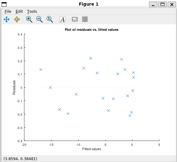
A few things worth knowing about what each plot reveals. The fitted plot is the most commonly used - if the residuals scatter randomly around zero with no visible curve or fan shape, the model assumptions are satisfied. The lagged plot helps detect autocorrelation (if residuals drift together, consecutive observations are correlated). The probability plot checks whether the residuals follow a normal distribution (they should fall near the straight reference line). The symmetry plot checks whether the residual distribution is symmetric around the median.

Here is what the fitted residual plot looks like:

n = 20;
X = [1:n; (1:n).^2]' / n;
y = X * [3; -1] + 0.2 * sin ((1:n)');
mdl = fitlm (X, y);
h = plotResiduals (mdl, 'fitted')

plotDiagnostics

plotDiagnostics visualises the observation-level influence statistics that live in mdl.Diagnostics. These help you find unusual observations - ones that are pulling the model disproportionately or that do not fit the pattern of the rest of the data.

plotDiagnostics (mdl)                ## default: leverage vs row number
plotDiagnostics (mdl, 'cookd')       ## Cook's distance vs row number
plotDiagnostics (mdl, 'covratio')    ## CovRatio vs row number
plotDiagnostics (mdl, 'dfbetas')     ## Dfbetas for each coefficient
plotDiagnostics (mdl, 'dffits')      ## Dffits vs row number
plotDiagnostics (mdl, 's2_i')        ## delete-1 variance vs row number
plotDiagnostics (mdl, 'contour')     ## standardized residuals vs leverage

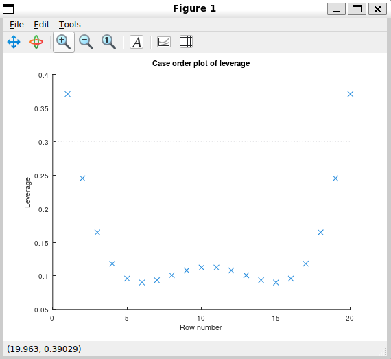
Each plot draws a reference line so you can immediately see which observations are worth a closer look:

• leverage - any observation above the line is sitting far from the centre of the data and has the potential to pull the model.
• cookd - any observation above the line is shifting the overall predictions more than typical.
• covratio - observations outside the two lines are affecting how confidently the coefficients are estimated.
• dfbetas - shows how much each observation moves each individual coefficient. One set of lines per coefficient.
• dffits - shows how much each observation shifts its own predicted value.
• s2_i - observations sitting well below the line were making the model’s error look larger than it really is.
• contour - puts leverage and residuals together on one plot with Cook’s distance curves overlaid, giving you the fullest picture of influence in a single view.

You can customise the marker appearance with the same Name-Value options as plotResiduals:

plotDiagnostics (mdl, 'cookd', 'Color', [1 0 0], 'Marker', 'o')

Here is what the leverage plot looks like for the default model:

h = plotDiagnostics (mdl, 'leverage')

plotEffects

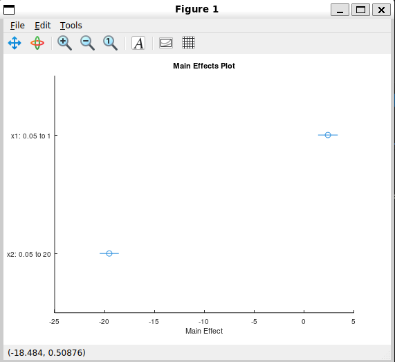
plotEffects shows how the predicted response changes as each predictor moves from its low value to its high value, while holding all other predictors fixed at their mean (or most frequent category).

This is a useful way to compare how much each predictor contributes to the model’s predictions. A predictor with a wide effect range matters a lot; one with a narrow range has little practical impact even if it is statistically significant.

plotEffects (mdl)          ## one horizontal bar per predictor
h = plotEffects (mdl)      ## get the graphics handles back
plotEffects (ax, mdl)      ## target a specific axes object

The chart is a dot-and-line plot. Each predictor gets one line. The centre dot is the predicted response when that predictor is at its mean and everything else is also at its mean. The line extends left and right to show the predicted response when that predictor is one standard deviation below and above its mean. For categorical predictors, the endpoints are the lowest and highest category levels instead.

Here is what it looks like:

h = plotEffects (mdl)

BIST Refactoring

This week we cleaned up and simplified the BIST (test) suite for the shared mdl object and a few related bugs we found along the way, instead of leaving lots of scattered, repeated tests.

Development Branch

All the code is on this branch: gsoc-2026-linearmodel

Next Steps

With the three plotting methods done, the remaining ones from the original list are:

• plotAdjustedResponse - plots the response against one predictor with the effect of all other predictors removed, so you can see that predictor’s relationship with the response in isolation.
• plotAdded - shows what one predictor adds to the model after everything else is already accounted for, the classic added variable plot.
• plotSlice - shows the predicted response as a function of each predictor individually, holding the others fixed, with sliders to move those fixed values interactively.
• plot - a simple scatter plot of the observed response against the fitted values.
• plotInteraction - shows how the effect of one predictor changes depending on the level of another, useful for spotting interaction effects visually.

After the plotting methods, the focus shifts to stepwiselm and CompactLinearModel.

Stay tuned for the next update!